Understanding the Graph of y = 3x + 1: A Complete Guide to Linear Functions
In the vast landscape of algebra and coordinate geometry, few concepts are as foundational and widely applicable as the graph of a linear equation. On top of that, the simple expression y = 3x + 1 is more than just a string of symbols; it is a precise mathematical recipe that describes a straight line on the Cartesian plane. Mastering how to interpret and construct this graph unlocks the ability to model countless real-world relationships, from calculating costs and speeds to understanding basic trends in data. This article will serve as your definitive guide to deconstructing, building, and understanding the graph of y = 3x + 1, transforming it from an abstract formula into a concrete visual tool That alone is useful..
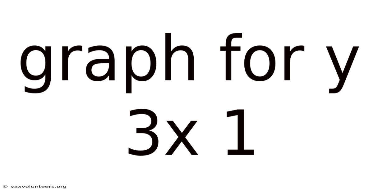
Detailed Explanation: Decoding the Slope-Intercept Form
The equation y = 3x + 1 is written in slope-intercept form, which is universally expressed as y = mx + b. This form is incredibly powerful because it reveals two critical characteristics of the line directly from the equation, without requiring any calculation. The first component is the slope (m), which in our equation is the number 3. The slope is the measure of the line's steepness and direction. It is defined as the ratio of the vertical change (rise) to the horizontal change (run) between any two points on the line. A slope of 3 means that for every single unit you move to the right along the x-axis (a run of +1), the corresponding y-value increases by 3 units (a rise of +3). This positive slope indicates the line ascends from left to right.
The second component is the y-intercept (b), which in our equation is the constant 1. So, the point (0, 1) is the y-intercept. Still, the y-intercept is the point where the line crosses the y-axis. Consider this: for y = 3x + 1, substituting x = 0 gives y = 1. This point serves as a crucial anchor or starting point for plotting the line. Since the y-axis is the line where x = 0, the y-intercept is simply the value of y when x is zero. The beauty of slope-intercept form is that it gives you a "plotting recipe": start at the y-intercept, then use the slope to find a second point, and finally draw a straight line through them Simple, but easy to overlook..
Step-by-Step: Plotting the Line y = 3x + 1
Creating an accurate graph is a systematic process. Follow these steps to plot y = 3x + 1 with precision.
Step 1: Identify the Slope and Y-Intercept. First, clearly label the components from your equation y = 3x + 1 That's the part that actually makes a difference..
- Slope (m) = 3. Remember, 3 can be written as the fraction 3/1, which explicitly shows rise/run.
- Y-intercept (b) = 1. This corresponds to the point (0, 1).
Step 2: Plot the Y-Intercept. On your coordinate plane (graph paper is ideal), locate the y-axis (the vertical line). Find the value 1 on this axis and place a solid dot at the point (0, 1). This is your first confirmed point on the line.
Step 3: Use the Slope to Find a Second Point. From your y-intercept (0, 1), apply the slope 3/1.
- Rise: Move up 3 units (since the rise is positive 3).
- Run: Move right 1 unit (since the run is positive 1). Starting at (0, 1), moving up 3 brings you to y = 4, and moving right 1 brings you to x = 1. You have now arrived at the second point (1, 4). Place another solid dot here. For greater accuracy, you can repeat this process from the y-intercept in the opposite direction: a rise of -3 and a run of -1 (down 3, left 1) would land you at the point (-1, -2). Plotting this third point is an excellent check on your work.
Step 4: Draw the Line. Using a ruler, draw a perfectly straight line that passes through all the plotted points (at least two are necessary, but three provides confirmation). Extend the line with arrows on both ends to indicate it continues infinitely. This completed line is the graphical representation of all solutions to the equation y = 3x + 1 That's the whole idea..
Real Examples: From Paper to the Real World
The abstract line on graph paper models tangible situations. In real terms, suppose a taxi service charges a flat "flag drop" fee of $1. Here, the total fare (y) depends on the miles (x). 00 (the base charge) plus $3.00 for every mile traveled. Think about it: the graph visually shows that traveling 0 miles costs $1, 2 miles costs $7, and 5 miles costs $16. The equation is Total Fare = 3 × (Miles) + 1, or y = 3x + 1. That's why the slope ($3/mile) is the rate of change. Consider a taxi fare calculator. The y-intercept ($1) is the initial charge the moment you step in. The line's constant steepness confirms the rate is fixed That alone is useful..
You'll probably want to bookmark this section.
Another example is in physics with constant velocity. That's why imagine a cyclist starting 1 meter ahead of a starting line (position = 1m at time t=0) and moving at a constant speed of 3 meters per second. The position (y) at any time (x in seconds) is y = 3x + 1. The slope (3 m/s) is the velocity. The y-intercept (1 m) is the initial position. The graph is a straight line because the velocity is unchanging. Any point on the line, like (4, 13), tells you that after 4 seconds, the cyclist is 13 meters from the origin.
Worth pausing on this one.
Scientific or Theoretical Perspective: The Cartesian Connection
The ability to graph y = 3x + 1 rests on the Cartesian coordinate system, invented by René Descartes. That said, this system merges algebra (equations) with geometry (shapes) by representing numbers as points on a plane using ordered pairs (x, y). A linear equation in two variables, like ours, defines a linear function.