Introduction
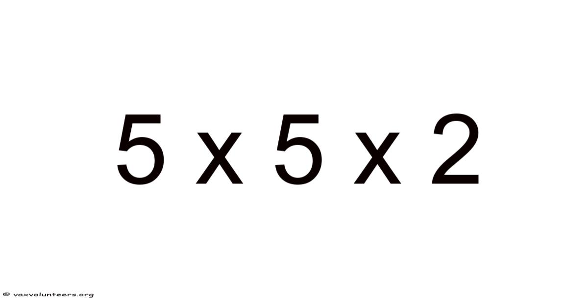
When you encounter a string of numbers linked by multiplication signs, such as .5 x .5 x 2, it may look like a simple arithmetic puzzle, but it actually opens the door to a broader understanding of how decimals interact, how order influences results, and why these operations appear in everyday calculations. This article treats .5 x .5 x 2 as the central keyword, dissecting its meaning, walking you through each computational step, and illustrating its relevance with concrete examples. By the end, you will not only know the numerical answer but also appreciate the underlying concepts that make this tiny expression a building block for more complex mathematical ideas.
Detailed Explanation
The expression .5 x .5 x 2 consists of three numeric terms connected solely by the multiplication operator. Each “.5” represents one‑half, a decimal notation for the fraction 1/2, while the final “2” is a whole number. In elementary arithmetic, multiplication is associative, meaning that the way we group the numbers does not affect the final product. This property allows us to compute the expression in any sequence, though following a left‑to‑right approach is often the most straightforward for beginners Simple, but easy to overlook..
Beyond the mechanics, the expression serves as a miniature model for scaling operations. Whenever a quantity is reduced to half and then multiplied by another factor, the result can either shrink further or expand, depending on the second multiplier. 5 x 2** belies its utility: it encapsulates the essence of repeated halving and subsequent scaling, a pattern that recurs throughout mathematics and its applications. In practical terms, understanding this helps in fields ranging from recipe adjustments to physics calculations involving proportional relationships. The simplicity of **.## Step‑by‑Step or Concept Breakdown
To demystify the computation, let’s break the process into clear, logical steps. 5 x .Each step builds on the previous one, ensuring that the reasoning remains transparent and easy to follow Not complicated — just consistent..
- Step 1 – Multiply the first two factors:
.5 x .5 equals 0.25 (or ¼). This is because half of a half is a quarter. - Step 2 – Multiply the result by the third factor:
0.25 x 2 yields 0.5 (or ½). Doubling a quarter restores us to one half.
A concise bullet‑point summary reinforces the flow:
- Multiply .5 by .5 → 0.25
- Multiply 0.25 by 2 → 0.5
By adhering to this step‑by‑step methodology, learners can avoid common pitfalls such as mis‑ordering operations or misplacing decimal points. The associative property guarantees that regardless of whether we compute (.Which means 5 x . Practically speaking, 5) x 2 or . 5 x (.5 x 2), the final product remains 0.5, but performing the operations sequentially aids comprehension, especially for those new to decimal arithmetic.
Real Examples Real‑world scenarios bring abstract numbers to life, and .5 x .5 x 2 appears in several practical contexts.
- Cooking and Recipe Scaling: Imagine a recipe that calls for ½ cup of sugar. If you halve the recipe (multiply by .5) and then double the resulting amount (multiply by 2), you end up with the original ½ cup, illustrating how scaling up and down can cancel each other out.
- Physics – Area Calculations: When computing the area of a shape that is scaled by a factor of .5 in one dimension and then expanded by a factor of 2 in another, the net effect on area is a multiplication of .5 × .5 × 2, resulting in a 0.5‑times original area. This demonstrates how combined scaling factors influence geometric properties.
- Probability – Independent Events: If an event has a probability of .5 (a coin toss landing heads) and you consider two independent such events, the combined probability of both occurring is .5 × .5 = .25. If a subsequent step doubles the odds (e.g., a bonus round), the final probability becomes .
Continuing the probability illustration, when the two independent 0.5‑chance events are followed by a factor that doubles the odds — such as a bonus round that awards a second chance — the calculation proceeds as follows:
- First, the chance that both initial events occur is 0.5 × 0.5 = 0.25 (25 %).
- Then, applying the doubling factor of 2 multiplies this result by 2, giving 0.25 × 2 = 0.5 (50 %).
Thus, the overall likelihood of success after the bonus step rises back to one‑half, illustrating how successive scaling can offset earlier reductions But it adds up..
The same pattern emerges in other domains. In finance, halving an investment and then restoring the original size with a 2× return yields the initial capital unchanged, a principle that underpins many risk‑management strategies. That's why in mechanical engineering, reducing a shaft’s diameter by half and subsequently increasing its length by twice the original dimension leaves the volume unaltered, which is crucial when designing components that must retain specific mass or stiffness characteristics. Even in computer graphics, applying a 0.5× scale to a texture in one axis and a 2× scale in another results in a net area that is exactly half of the original, a fact that designers exploit to conserve memory while preserving visual fidelity.
The short version: the compact expression .And 5 × . 5 × 2 serves as a clear illustration of how repeated halving followed by a doubling can neutralize each other, producing a net factor of 0.5. Recognizing this relationship equips learners and practitioners with a versatile tool for adjusting quantities, interpreting proportional changes, and solving problems across mathematics, science, and everyday decision‑making.
You'll probably want to bookmark this section Worth keeping that in mind..
This multiplicative interplay extends further into nuanced scenarios. Consider project management, where task estimates might be halved due to initial optimism, only to face a 2× delay due to unforeseen complexities. Even so, the net effect on the timeline isn't neutral; it reflects the 0. On the flip side, 5 × 2 = 1 factor applied to the original estimate, resulting in no net change to the baseline, though the path to completion was fraught. Similarly, in pharmacokinetics, halving a drug's dosage (.5×) and then doubling the frequency of administration (2×) maintains the same total daily drug exposure (AUC), crucial for maintaining therapeutic levels while managing side effects Simple as that..
Even in ecological modeling, population dynamics illustrate this principle. If a population is reduced by half due to a disease (.5×) and then experiences a growth spurt doubling its size (2×), the net effect is a return to the original population size, assuming no other factors intervene. This simple calculation helps predict population rebounds after environmental shocks.
The universality of .5 × .Practically speaking, 5 × 2 = 0. Worth adding: 5 underscores a fundamental truth about proportional relationships: sequential multiplicative changes compound predictably. Recognizing this allows for rapid mental estimation and scenario testing across countless applications. It transforms abstract numbers into tangible tools for predicting outcomes in resource allocation, system design, risk assessment, and scientific modeling.
To wrap this up, the seemingly simple sequence of halving and then doubling, encapsulated mathematically as .5 × 5 × 2 = 0.5, reveals a profound and versatile principle. It demonstrates how multiplicative factors interact, often neutralizing or compounding effects in predictable ways. From the kitchen to the cosmos, this understanding provides a foundational lens for interpreting change, optimizing processes, and making informed decisions. Mastering this concept empowers individuals to handle proportional complexities with clarity and confidence, proving that even the most basic mathematical operations can get to deep insights into the interconnected nature of our world Small thing, real impact..
